How this works
There are 24 projects on this page, in two groups. The first fifteen are built on things the course covers. They run on public data or on hardware the lab already has, and each one has a baseline we expect you to beat and a number you have to report. The last projects are harder. Open about the method implementation & ideation, the answer might be “no” that this doesn’t work, and if it goes well you might have a paper too.
Neither group is worth more marks. A grounded project done properly (ablations run, failure cases found and explained) beats an ambitious one that ends in a demo video and a vibe.
Got your own problem? Even better. Read your own project before you fill the form.
Teams
Two or three people. Three is fine on any project and expected on the hardware ones, because someone has to hold the robot while someone else reads the terminal. We grade a team of three against a bigger scope than a team of two, so say what that bigger scope is in your timeline document.
Find your own team. If you don’t have one by Sep 8, tell a TA and we’ll pair you with whoever else is in the same spot.
More than one team can take the same project. If eight teams want the feed forward at scale we’ll ask some of you to move, so put your preferences wisely in the form.
Timeline
| Item | Date |
|---|---|
| Project list released | Sep 5 |
| Team and project preference form due | Sep 13 |
| Mentor assignment posted | Sep 14 |
| Timeline document due | Sep 17 |
| Mid submission due | Oct 26 |
| Final submission due | Nov 23 |
| Demos | Nov 26 |
The form will be shared soon on Moodle. It asks for your team, a first and second choice of project, and a first and second choice of mentor.
Mentors
Every team gets a TA mentor. Before you fill the form, come talk to us. Tell us what you want to build, ask us what we’ve worked on. Tarun, Krish and Akash have worked on fairly different things, and the whole point of the conversation is figuring out whose experience is closest to your project.
Put a first and second choice on the form. You’ll usually get your first choice. If a mentor is oversubscribed, or if your project is honestly closer to what a different TA has done, we’ll reassign, and it goes to whoever has spent the most time on that kind of problem. We sort this out among ourselves and post it on Sep 14, three days before the timeline document is due.
What does a mentor do? Reads your timeline document, is the person you message when the project stalls, grades your submissions. Book time with them in September. Half an hour in week two with someone who has already debugged your pipeline saves you three weeks in November.
Submissions
Everything goes on Moodle. The project is 30% of the course, split as follows.
| Component | Weight | Due |
|---|---|---|
| Timeline document | 5% | Sep 17 |
| Mid submission | 7% | Oct 26 |
| Final submission and demo | 18% | Nov 23, demos Nov 26 |
The timeline document is two pages: team, project, mentor, the dataset or robot you’re running on, the baseline you’re comparing against, the metric you’re reporting, and who does what by when. No metric, we send it back.
The mid submission is code, data and results so far, a short presentation, and a two to three page LaTeX report. By Oct 26 the baseline has to run end to end on your data, even if your own method doesn’t work yet. Working baseline, broken method: fine. Neither: not fine.
The final submission is code, data, results, a presentation with a live or recorded demo, and a six to eight page LaTeX report. Put the ablations in. Put the failure cases in. Negative results are fine as long as you measured them and can say why they happened.
Grounded projects
You can start any of these the day you’re allotted it. The baseline already exists, so you can measure against it from week one.
1. LIDAR odometry and mapping with loop closure
Build a LIDAR SLAM pipeline end to end on a KITTI odometry sequence. Voxel downsample, estimate normals, register scan to map with point to plane ICP, pick keyframes, propose loop closures when you revisit a place, solve the pose graph in Ceres or g2o. The front end is done by day three. The back end is where you find out whether your map has one corridor in it or two.
Numbers we want: KITTI translational and rotational drift over the 100 to 800 m subsequences, and absolute trajectory error, both before and after the pose graph solve. Plus the same map rendered before and after loop closure, and how many loop candidates you proposed vs how many you accepted (that ratio says a lot about your detector).
References: KITTI odometry benchmark, KISS-ICP, LeGO-LOAM, Grisetti et al., graph based SLAM tutorial.
2. Occupancy mapping that survives moving obstacles
Log odds occupancy grid, inverse sensor model, lecture 8. It’s quick to get running. Keeping it clean is the problem: every car and every person that walks past leaves a trail of occupied cells that stick around long after the object is gone. So implement the mapping, then implement something that clears the trails. Ray cast through free space, decay the log odds, filter moving points before they enter the map, or all three and compare.
Evaluate on a sequence with moving object labels (SemanticKITTI has them). Report IoU of your static map against the ground truth static map, the number of cells still occupied where nothing static exists, and how both change as you turn the decay up. At some decay rate you start deleting real walls the robot hasn’t looked at for a while, and we’d like to know where that rate is.
References: Thrun, Burgard and Fox, ch. 9; SemanticKITTI; nuScenes; Stachniss, occupancy grid maps.
3. LIDAR to camera calibration with an error budget
Estimate the 6 DoF transform between a LIDAR and a camera. Start target based (a checkerboard or a few planes give you 3D to 3D or 3D to 2D correspondences) and minimise reprojection error. Then go targetless: image edges against depth discontinuities in the scan. Honestly the pipeline isn’t the project. The error analysis is. How does the estimate degrade as you throw away correspondences? How far off can the initial guess be before the optimiser wanders off? Which of the six parameters does your data barely constrain?
Report reprojection error of LIDAR points into the image against the dataset’s published extrinsics, with degradation curves against number of correspondences and against initial offset. Show the coloured point cloud. Show a bad one too.
References: Dhall et al., LiDAR camera calibration using 3D-3D point correspondences; direct_visual_lidar_calibration; Awesome LiDAR camera calibration.
4. Camera calibration you wrote yourself
Your task is to build a camera calibration pipeline from scratch. Start with a standard ChArUco board: detect its corners, estimate one homography per view, use Zhang’s planar method to recover the camera intrinsics, and refine the intrinsics, poses and radial distortion by minimizing reprojection error. Compare your result against OpenCV using the same images.
Once the pipeline works, apply it to the custom ChArUco board provided in the lab. Unlike a regular board, this target contains missing regions and large cut-outs, so your method must use marker IDs and the known board geometry to correctly establish correspondences when only part of the board is visible.
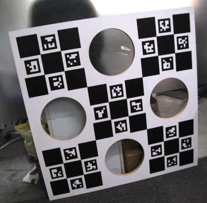
Report focal length, principal point, distortion and reprojection error against OpenCV, and study how the estimates change as you go from 3 images to 30. Compare the standard and custom boards, then repeat the experiment using mostly fronto-parallel views. Explain why this configuration makes focal length poorly constrained even when the reprojection error remains small.
References: Zhang, a flexible new technique for camera calibration; Hartley and Zisserman, ch. 6 and 7; OpenCV ChArUco; OpenCV calibration.
5. Structure from motion ending in bundle adjustment
Incremental SfM over 30 to 100 images of one scene. Features, matching, essential matrix and relative pose for a seed pair, triangulate, PnP with RANSAC for each new view, retriangulate as the model grows, bundle adjust in Ceres with a Huber loss.
Report mean reprojection error before and after each BA, camera poses against COLMAP on the same images, how many points survive the cheirality and reprojection checks, and how far the reconstruction bends if you skip BA entirely. Also pick the seed pair badly on purpose once (two nearly identical views) and see how well the thing recovers.
References: Hartley and Zisserman, ch. 9 to 11; Triggs et al., bundle adjustment, a modern synthesis; COLMAP; Ceres bundle adjustment example.
6. Dense stereo depth, three ways
Rectify a pair, then compute disparity three ways: block matching over a cost volume, semi global matching, and a learned network off the shelf. Same rectified input to all three. Turn disparity into depth, depth into a point cloud.
Report the fraction of pixels with disparity error above 2 px on Middlebury or KITTI 2015, runtime per pair, and (this is the important part) error split by region: textureless walls, occlusion boundaries, repetitive structure, thin things like poles. The average hides exactly where each method breaks, so don’t only give us the average.
References: Middlebury stereo; KITTI stereo 2015; Hirschmuller, semi global matching, CVPR 2005; slambook-en, ch. 4.
7. Moving object detection from epipolar violations
Between two frames, a static point has to sit on its epipolar line. A point that doesn’t is either a bad match or something moving. So estimate F from the static correspondences, compute Sampson distance for every tracked point, and separate movers from outliers. Then the annoying case: an object moving along its own epipolar line. That’s the car in front of you, going the same way you are, and you need a second cue for it (depth consistency, or the trifocal constraint over three frames).
Report precision and recall of moving points against KITTI tracking labels, and how they move with the threshold, the number of frames used, and the vehicle speed. Give the car in front its own table.
References: KITTI tracking; Hartley and Zisserman, ch. 9 and 15; the moving object detection paper on Moodle.
8. ICP variants and where they stop converging
Point to point, point to plane, GICP, NDT, all on the same scan pairs. Final registration error is the boring number. What we want is the convergence basin: sweep the initial transform over a grid of rotation and translation offsets, run every variant from every start, and plot the fraction that ends up at the right answer. Then add outliers, cut the overlap, and watch the basin shrink.
Report the basin plots per variant, iterations to convergence, time per iteration, and the overlap fraction where each one gives up. Do it on indoor scans and on KITTI scans, because the ranking isn’t the same indoors and out.
References: Rusinkiewicz and Levoy, efficient variants of ICP; Segal, Haehnel and Thrun, generalized ICP, RSS 2009; Open3D registration; Stachniss, ICP with unknown data association.
9. A pose graph solver written from scratch
Gauss Newton and Levenberg Marquardt for pose graph optimisation in SE(2) and SE(3), written by you. Analytic Jacobians. A rotation parameterisation the solver can actually handle (a local perturbation on the manifold, not raw Euler angles, lecture 19 covers why). Exploit the sparsity of the information matrix and solve with sparse Cholesky. Then break it: bad initialisation, and one wrong loop closure with a very confident information matrix.
Report final chi squared, iterations and wall clock against g2o and Ceres on the standard datasets (Intel, MIT Killian Court, sphere2500, torus), and trajectory error under a growing fraction of false loop closures, with and without a Huber loss or switchable constraints. If your solver and g2o disagree somewhere, chase it down. Don’t round it off.
References: Grisetti et al., graph based SLAM tutorial; Kuemmerle et al., g2o; Suenderhauf and Protzel, switchable constraints, IROS 2012; pose graph datasets.
10. AprilTag mapping and localisation
Detect AprilTags, get each tag’s 6 DoF pose relative to the camera, build a factor graph where the variables are camera poses and tag poses and the factors are the detections. Solve it in GTSAM or g2o for a consistent tag map. Then freeze the map and run localisation only: given the tags you can see right now, where is the camera?
Report tag positions against hand measured ground truth, localisation error against a reference trajectory, how fast localisation runs, and pose error against tag distance and viewing angle. One thing to know going in: a single small tag seen nearly head on has two valid poses, and the detector flips between them. Don’t filter that out of your plots. Show it, then deal with it.
References: AprilTag; Wang and Olson, AprilTag 2, IROS 2016; GTSAM; Kaess et al., iSAM2, IJRR 2012.
11. Place recognition judged by what it does to the map
Loop closure detectors get reported with a precision recall curve, and that’s where most papers stop. But one false positive with a confident information matrix folds your map in half, and the curve doesn’t tell you how close you are to that. So: compare a bag of words detector, a learned global descriptor, and a LIDAR descriptor on the same sequences, then push each one’s output through the same pose graph backend.
Report the PR curves, sure. Then report the absolute trajectory error of the map built from each detector, and how many false positives the backend tolerates before the map breaks, with and without an outlier tolerant loss.
References: Galvez-Lopez and Tardos, DBoW2; Arandjelovic et al., NetVLAD; Kim and Kim, Scan Context, IROS 2018; Cummins and Newman, FAB-MAP, IJRR 2008.
12. Stereo visual odometry with a sliding window
Lucas Kanade tracking across frames, triangulate from the stereo pair, PnP with RANSAC for motion, then local bundle adjustment over a sliding window of keyframes. Keyframe spacing, window length and how aggressively you cull features are the three knobs. They decide whether you drift a metre or fifty.
Report translation and rotation drift on KITTI with and without the sliding window, error against keyframe spacing, runtime per frame. Then record your own sequence on the lab stereo camera, run the same code, and tell us where the numbers differ from KITTI and what in your recording caused it (usually exposure, or the rolling shutter).
References: KITTI odometry; slambook-en, ch. 6 to 9; ORB-SLAM3 as a reference implementation to read.
13. Merging maps recorded on different days
Two point cloud maps of the same corridor or car park, recorded on different days, from different start points, with stuff moved around in between. Find the transform between them with no common start pose: FPFH features plus RANSAC (or a learned descriptor), then ICP to refine. Merge them. Then figure out what changed.
Report registration success rate over many session pairs, residual after refinement, runtime, and how it degrades as the overlap drops. For the change detection half, keep a list of what you moved while recording and report what you found against it. A system that registers 90% of the time and one that registers every time are different systems, so tell us about the 10%.
References: Rusu et al., FPFH, ICRA 2009; Open3D global registration; Zhou, Park and Koltun, fast global registration, ECCV 2016; Fehr et al., TSDF based change detection, ICRA 2017.
14. Monocular visual odometry with the scale put back
Matching, essential matrix, pose recovery, triangulation: you get a trajectory up to scale, and the scale drifts. Fix it with something you can measure. A known camera height above a ground plane fitted per frame, a known object size, or wheel odometry over a short window. Then see how long the fix holds.
Report ATE after a similarity fit to ground truth, for the scale free baseline and for each constraint. Plot estimated scale over time against ground truth, so we can see the drift before one global fit at the end hides it. How often does the ground plane fit fail, and what does the trajectory do when it does?
References: Nister, an efficient solution to the five point relative pose problem, TPAMI 2004; slambook-en, ch. 6; Scaramuzza and Fraundorfer, visual odometry tutorial, RA-M 2011; KITTI odometry.
15. Four map representations, measured
One scanned environment, stored four ways: voxel grid, octree, TSDF, and a mesh pulled out of the TSDF. Write the TSDF integration yourself. That’s where the parameters that matter live (truncation distance, weighting, voxel size).
Report memory at a few resolutions, time to integrate a scan, time to answer an occupancy query and a nearest surface query, and surface error against a reference scan. And report the resolution where each representation stops fitting in the RAM a robot actually has onboard, because that decides what you can deploy and reconstruction error alone won’t tell you.
References: OctoMap; Curless and Levoy, a volumetric method for building complex models from range images, SIGGRAPH 1996; Newcombe et al., KinectFusion, ISMAR 2011; Open3D TSDF integration; Oleynikova et al., Voxblox, IROS 2017.
Open-ended projects
These are harder. The method isn’t settled, the compute is bigger, and some of them will come back negative. That’s fine. Measure it, explain it, full marks. Take one of these if you want the project to end in a paper. The reporting bar is the same as above, so read submissions again first.
16. Multi-robot mapping under a bandwidth budget
Two or three robots map the same building and merge their maps. Each runs its own SLAM. The question is what they send each other. Sending full point clouds works and is useless outside a lab. So design the exchange: compact descriptors for place recognition first, then relative pose measurements only for the candidates that match, then a joint pose graph solve. And handle the case where the maps don’t overlap yet and the merge has to wait.
Report trajectory and map error against a single robot covering the same area, total bytes exchanged, and error as a function of a hard bandwidth cap. Then inject one wrong inter robot loop closure and report what it does to both maps, since that’s the failure a single robot never sees.
References: Lajoie and Beltrame, Swarm-SLAM; Tian et al., Kimera-Multi; Choudhary et al., distributed mapping with privacy and communication constraints, IJRR 2017.
17. Feed forward geometry at kilometre scale
VGGT gives you pointmaps and poses for a few dozen frames in one forward pass. A KITTI sequence is 4000 frames. So the obvious move is to chunk it: run the model over overlapping windows, register each window to the next with a Sim(3) (every window has its own arbitrary scale), close loops with the encoder’s global feature, and optimise a pose graph. VGGT-Long does exactly this and gets kilometre scale trajectories out of a monocular camera. Reproducing it is the easy half of this project.
The hard half is the pose graph. What information matrix goes on the edge between two windows? These models output a confidence per pixel, and it’s not obvious that those confidences track the actual error. So check. Compare predicted confidence against measured depth and pose error on sequences with ground truth. Are they calibrated? If they aren’t (our bet), fit a calibration, derive per edge covariances from it, hand those to the backend, and see whether the trajectory improves over uniform weights and over VGGT-Long’s own weighting. Same question for the loop closure edges, which are the ones that fold the map when they’re wrong.
Numbers: ATE against sequence length on KITTI odometry, Waymo and TUM RGB-D, compared with VGGT-Long, MASt3R-SLAM, DROID-SLAM and ORB-SLAM3. Calibration curves (predicted against empirical error) for depth and for relative pose, before and after your calibration. ATE with uniform weights, raw confidence weights and calibrated weights. Peak GPU memory and frames per second, since the whole reason to chunk is that the sequence doesn’t fit.
Bonus: swap VGGT for a streaming model (CUT3R, StreamVGGT) and find out whether a persistent state removes the need for chunking or just hides the drift.
References: Deng et al., VGGT-Long; VGGT; Murai, Dexheimer and Davison, MASt3R-SLAM, CVPR 2025; Wang et al., CUT3R, CVPR 2025; Zhuo et al., StreamVGGT; Structure from Attention, on what these networks attend to; KITTI odometry.
18. Metric depth priors inside monocular SLAM
Monocular SLAM has no scale and initialises badly. Monocular metric depth networks (UniDepth, Metric3D v2, Depth Anything V2 with the metric head) give you a dense depth map per frame with actual metres attached. So feed one into a monocular SLAM system. There are three places it can go: initialisation, the tracking cost, and a prior in the backend. Which one actually helps? Not obvious in advance.
Report ATE and scale error against the monocular baseline and against the RGB-D upper bound on the same sequences, plus map density. Then weight the depth term by the network’s own confidence and see if that helps. A depth prior that’s confidently wrong on a reflective floor should show up in your error plots, so don’t smooth it out.
References: Piccinelli et al., UniDepth, CVPR 2024; Metric3D v2; Depth Anything V2; DROID-SLAM; ORB-SLAM3.
19. Distilling a vision model into a LIDAR network
Image encoders trained on hundreds of millions of images know things about the world that a LIDAR network trained on point clouds alone never picks up. Take a dataset with synchronised camera and LIDAR, project image features onto points using the extrinsics, and train a point cloud network to predict those features. What you end up with is a LIDAR only network with image derived semantics, and it keeps working when the camera is blinded by sun or rain.
Report linear probe and fine tuned performance on LIDAR semantic segmentation against a randomly initialised network and against the same network pretrained with a point cloud only objective. Report the label efficiency curve at 1%, 10% and 100% of the labels, since the whole argument for pretraining lives at the low label end.
References: Sautier et al., SLidR, CVPR 2022; Puy et al., three pillars improving vision foundation model distillation for LiDAR, CVPR 2024; nuScenes; SemanticKITTI; Waymo Open Dataset.
20. Feature extractors for visual odometry, measured end to end
Take one visual odometry pipeline and swap the front end between ORB, SIFT, SuperPoint with LightGlue, ALIKED, and dense matches from MASt3R. Everything downstream stays fixed so you’re measuring the extractor and nothing else. Building that fixed backend is most of the work, to be honest.
Report trajectory error, tracking failures, matches per frame, inlier ratio after RANSAC, and runtime on EuRoC and KITTI. Then break the sequences on purpose (motion blur, low light, blank walls) and report it all again. Learned extractors usually win on average and lose somewhere specific. Where?
References: DeTone et al., SuperPoint; Lindenberger et al., LightGlue, ICCV 2023; Zhao et al., ALIKED, TIM 2023; EuRoC MAV.
21. Lifelong mapping and 3D change detection
You build a map once and then it rots. Furniture moves, doors close, boxes appear. Build a system that loads last week’s map, relocalises in it with no initial pose, works out what changed, and updates the map without rebuilding it. The two hard parts are relocalising from cold and deciding whether a discrepancy is a real change or a sensor artefact.
Record the same area over at least five sessions across two weeks. Write down every change you make, because that log is the only ground truth you’ll have. Report relocalisation success rate and time from cold start, precision and recall of detected changes against your log, and map size across sessions. If map size grows every session, you’re not updating the map. You’re hoarding every version of the room it has ever seen.
References: Fehr et al., TSDF based change detection, ICRA 2017; Biber and Duckett, dynamic maps for long term operation, RSS 2005; Krajnik et al., FreMEn, T-RO 2017; OctoMap.
22. Radio fingerprints fused with visual odometry
Big open indoor spaces are where LIDAR and visual SLAM both fall over. The walls are too far away for the LIDAR and every corridor looks like every other corridor to the camera. WiFi and BLE signal strength has the opposite character: low rate, noisy, and globally distinctive. So build a fingerprint map of received signal strengths over a known floor plan, then fuse it with visual odometry in a particle filter or a factor graph. The odometry supplies the motion, the radio supplies the global fix.
Report position error against a ground truth trajectory for VO alone, radio alone, and the fusion. Report time to recover after you kidnap the robot. And report what happens when a third of the access points are switched off between mapping and localisation, because in a real building they will be.
References: Thrun, Burgard and Fox, ch. 8, Monte Carlo localisation; Double-Layer Soft Data Fusion for Indoor Robot WiFi-Visual Localization; LRF-WiVi, a WiFi and visual indoor localization method based on low rank fusion.
23. Radar and camera fusion for point cloud densification
Automotive radar returns tens of points per sweep. A LIDAR returns a hundred thousand. But the radar keeps working in fog, rain and direct sun. Take synchronised radar and camera data, calibrate the extrinsics, and train or deploy a model that predicts a denser point cloud from the sparse radar plus the image. Then check whether the extra density actually bought anything downstream.
Report Chamfer distance of the densified cloud against a LIDAR scan of the same scene. Then run a LIDAR object detector on the densified cloud and compare it to the same detector on raw radar and on real LIDAR. Split all of it by clear and adverse weather. The clear weather number will look disappointing. The adverse weather number is why you did this.
References: Prabhakara et al., RadarHD, ICRA 2023; nuScenes radar sweeps; RADIATE; Oxford Radar RobotCar.
24. Monocular bird’s eye view maps for local planning
A forward facing image is hard to plan in. A top down map of the same scene is easy. Networks in the lift splat family predict a bird’s eye view semantic map from camera images by lifting image features into 3D and splatting them onto the ground plane. Deploy one, turn its output into a costmap, and drive a local planner from it.
Report IoU of the predicted BEV against a ground truth occupancy map from LIDAR, then report what the planner does with it: collision rate, path length against a LIDAR costmap baseline, and the distance at which the network stops getting free space right. Then accumulate predictions over time with odometry, and report both again.
References: Philion and Fidler, Lift, Splat, Shoot, ECCV 2020; Li et al., BEVFormer, ECCV 2022; Harley et al., Simple-BEV, ICRA 2023; nuScenes.
Your own project
A problem you found yourself beats anything on this page. Bring one from a lab you work in, a paper you read and disagreed with, a robot you already have access to. The list exists so nobody is stuck without a starting point, not because these are the 24 good ideas.
Write the proposal in the same shape as a timeline document: the problem, the data or robot, the baseline, the metric, and why a semester is enough. Send it to a TA before Sep 10 so we can account for it when assigning mentors. If it uses none of the geometry from this course we’ll send it back with a suggestion for how to bring it closer.
If you want the project to end in a paper, say so in the timeline document. A semester is enough for a paper or a workshop submission. Pick the evaluation the venue expects (public benchmark, named metric, ablations against a baseline) from day one so you aren’t bolting it on in November. We’ll read drafts.